CNN初解
首先,神经网络(Neural Networks)并不复杂,仅仅是一个专业词汇(唬人词汇),事实上,它远比想象中的要简单很多。
前置需求:一点点线性代数,一点点Python基础(如果都不了解,也能看懂大概)。
1. 初识神经网络(Neural Networks)
1.1 建立模块:神经元(Neurons)
首先神经网络的基本单元就是”神经元(Neurons)”。一个神经元的构成,首先有多个输入,然后对多个输入进行一些数学的运算,最后得到一个输出。 下图是一个典型的2个输入的神经元。
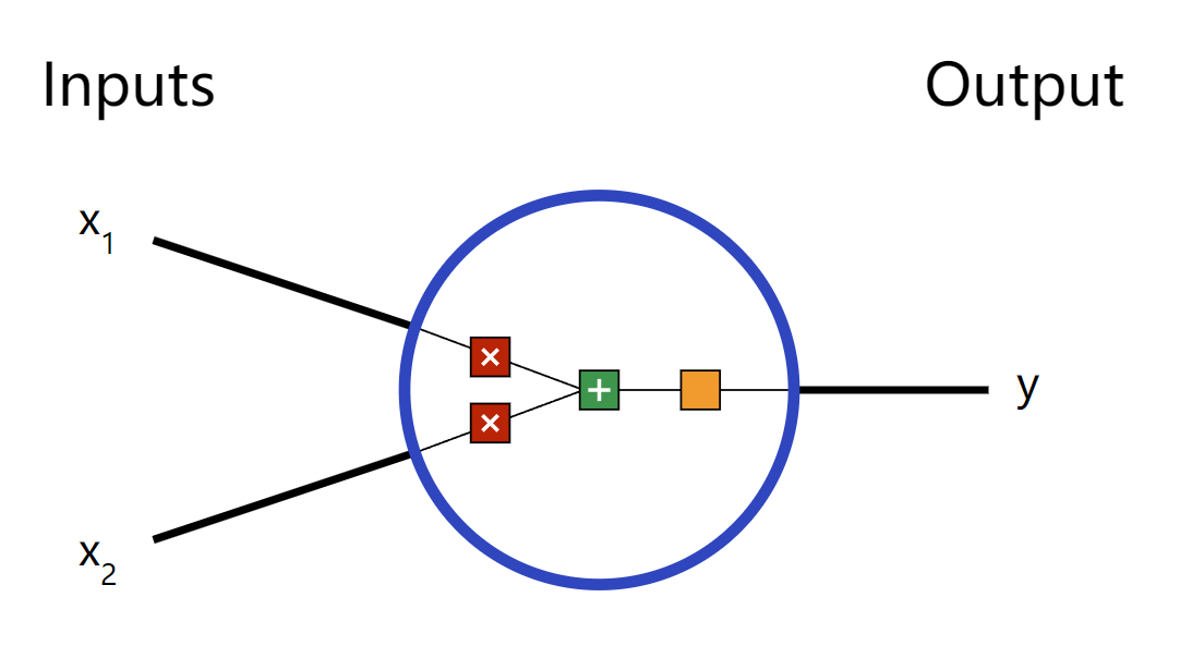
神经元中发生了三件事情:
首先,每个输入乘以一个权重(Weight):(图中红色方块)
$$
x_1 \rightarrow x_1 * w_1 \
x_2 \rightarrow x_2 * w_2
$$然后,所有的乘了权重之后的输入加到一起,并再加上一个偏置(bias)b:(图中绿色方块)
$$
(x_1 * w_1) + (x_2 * w_2) + b
$$
偏置b在此图中没有画出,后续学习中,可以理解偏置b就是一个权重固定为1的输入,有的教材中就将偏置b,直接等效为一个$$x_0$$乘以一个固定权重为1的输入
$$
(x_0 * 1) + (x_1 * w_1) + (x_2 * w_2)
$$最后,加到一起的和,经过一个激活函数:(图中橙色方块)
$$
y = f(x_1 * w_1 + x_2 * w_2 + b)
$$
这个激活函数主要作用是将一个无界限的输入(多个输入乘以权重相加后,是一个没有确定的界限的值),变为具有良好、可预测形式的输出。如下图的例子,就是一个常用的sogmoid激活函数(当然还有很多其它类型的激活函数,这里不进一步展开)。

这个sigmoid激活函数的输出范围是(0,1)。简单来说,这个激活函数的作用就是将一个可能为$$(-\infty, +\infty)$$范围的输入值(横坐标),转化为(0,1)的输出值(纵坐标)。输入越小的负数,经过sigmoid函数后,输出越接近于0;输入越大的正数,经过sigmoid函数后,输出越接近于1。
一个简单的例子
假设我们有一个神经元,具有2个输入,1个输出,使用sigmoid作为激活函数,具体的参数如下:
$$
w = [0,1] \
b = 4
$$
其中$$w=[0,1]$$只是$$w_1 = 0, w_2 = 1$$的向量写法。
现在我们给神经元一个输入向量$$x = [2,3]$$。我们使用更简洁的点乘(dot product)来表示:
$$
\begin{align}
(w \cdot x) + b &= ((x_1 * w_1) + (x_2 * w_2)) + b \
&= 0 * 2 + 1 * 3 + 4 \
&= 7
\end{align}
$$
$$
y = f(w \cdot x + b) = f(7) = 0.999
$$
输入向量$$x = [2,3]$$经过神经元后,得到0.999的输出。就是这么简单,这种向前传递输入(图中是从左向右传递),得到输出的过程称为前馈(feedforward)。
编写一个简单的神经元
我们使用Python中的Numpy包,它是一个很流行和强大的矩阵计算库,可以极大的方便进行数学矩阵运算。
1 | import numpy as np |
以上的python代码,就是上面举例子的代码实现,得到了相同的结果0.999。
1.2 多个神经元组合成一个神经网络
神经网络只不过是一堆连接在一起的神经元。下面就是一个简单的神经网络的样子(因为只有从左到右的传输,也叫前馈神经网络):
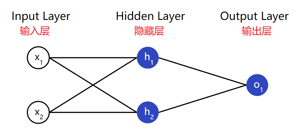
这个神经元有三层,第一层为输入层,具有两个输入,无神经元;第二层为隐藏层,具有两个神经元$$(h_1, h_2)$$;第三层为输出层,具有一个神经元$$o_1$$。注意这里$$o_1$$的两个输入是来自隐藏层的$$(h_1, h_2)$$–我们就叫这是一个网络。
注意:隐藏层是输入层(第一层)和输出层(最后一层)中间的任何一层。也就是说隐藏层可以有多层。
例子:一个简单的前馈神经网络
让我们使用上图的网络,并假设所有神经元具有相同的权重$$w = [0,1]$$,相同的偏置$$b = 0$$,相同的sigmoid激活函数。最后让$$(h_1, h_2, o_1)$$代表对应神经元的输出。
如果我们给定输入$$x = [2,3]$$,神经网络是怎么运转的呢?
$$
\begin{align}
h_1 = h_2 &= f(w.x + b) \
&= f((0 * 2) + (1 * 3) + 0) \
&= f(3) \
&= 0.9526
\end{align}
$$
$$
\begin{align}
o_1 &= f(w.[h_1, h_2] + b) \
&= f((0 * h_1) + (1 * h_2) + 0) \
&= f(0.9526) \
&= 0.7216
\end{align}
$$
因此,我们得到了输入$$x = [2,3]$$经过神经网络后,得到输出为0.7216。这是简单易懂的过程。
神经网络可以有任意数量的层,这些层中可以有任意数量的神经元。但基本思想保持不变:通过网络中的神经元向前馈送输入,在最后获得输出。为简单起见,在本文的其余部分,我们将继续使用上图的网络。
编写:一个简单的前馈神经网络
我们将上面前馈神经网络的例子,通过python代码呈现出来:
1 | import numpy as np |
最后得到相同的输出结果0.7216
1.3 训练一个神经网络,第一部分
我们假设有如下的测量参数:
| Name | Weight (lb)(磅) | Height (in)(英寸) | Gender |
|---|---|---|---|
| Alice | 133 | 65 | F |
| Bob | 160 | 72 | M |
| Charlie | 152 | 70 | M |
| Diana | 120 | 60 | F |
让我们来训练网络,通过给定体重和身高,来预测某人的性别:
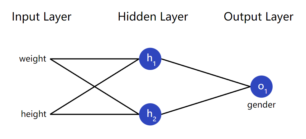
这里假设男生输出0,女生输出1,以及其它测量参数如下(这里选体重和身高随意选择了一个合适的值135磅和66英寸,这两个值也可以调整,主要是方便运算):
| Name | Weight (minus 135) | Height (minus 66) | Gender |
|---|---|---|---|
| Alice | -2 | -1 | 1 |
| Bob | 25 | 6 | 0 |
| Charlie | 17 | 4 | 0 |
| Diana | -15 | -6 | 1 |
表格中的体重和身高是减去合适的值(自己随意定)之后的值,比如Alice的体重-2,是由133(Alice自己的体重)减去135(体重中位数)得到的-2。
损失函数(Loss Function)
在开始训练神经网络之前,我们还需要一种方法来量化它做得有多“好”,以便它可以尝试做得“更好”。这就是损失函数的由来,也可以简称为损失(Loss)。
这里,我们使用均方差(Mean Squared Error, MSE)作为损失函数来衡量网络的好坏。
当然还有很多其它的损失函数,比如交叉熵(Cross Entropy)详见:常见损失函数介绍
均方差(MSE)损失函数:
$$
MSE = \frac{1}{n} \sum_{i = 1}^{n} (y_{true} - y_{pred})^2
$$
其中,$$n$$是样本的个数,这里是4(4表示Alice, Bob, Charlie, Diana);$$y$$表示性别,其中$$y_{true}$$表示真实的性别(比如Alice的$$y_{true} = 1$$),$$y_{pred}$$表示神经网络预测给出的性别。
上述公式中$$(y_{true} - y_{pred})^2$$是我们熟知的平方误差(squared error)。我们的均方差损失函数就是取所有平方误差的平均值(因此得名均方差)。所以我们的预测越好,我们的损失(均方差)就越低!
更好的预测 = 更低的误差(更小的均方差)
训练一个好的神经网络 = 让神经网络的损失尽量小
例子:均方差损失函数
这里先假设,我们神经网络的输出一直为0,换句话说,就是让神经网络一直预测这个人为男生,最后的损失应该是什么?
| Name | $$y_{true}$$ | $$y_{pred}$$ | $$(y_{true} - y_{pred})^2$$ |
|---|---|---|---|
| Alice | 1 | 0 | 1 |
| Bob | 0 | 0 | 0 |
| Charlie | 0 | 0 | 0 |
| Diana | 1 | 0 | 1 |
$$
MSE = \frac{1}{4}(1 + 0 + 0 + 1) = 0.5
$$
编写:均方差损失函数
1 | import numpy as np |
如果有疑惑,也可以看看numpy的官方教程:quickstart
1.4 训练一个神经网络,第二部分
当了解到损失函数后,我们现在有了一个清晰的目标:让神经网络的损失最小。
然后前面我们已经知道改变神经网络的权重和偏置,就可以影响神经网络的输出(预测),但是应该怎么来减少损失呢?
这部分会有一点点多变量微积分。如果不感兴趣,可以直接跳过数学计算部分。
为简单起见,让我们假设数据集中只有 Alice:
| Name | Weight (minus 135) | Height (minus 66) | Gender |
|---|---|---|---|
| Alice | -2 | -1 | 1 |
均方差损失就只是Alice的平方误差:
$$
\begin{align}
MSE &= \frac{1}{1} \sum_{i = 1}^{n} (y_{true} - y_{pred})^2 \
&= (y_{true} - y_{pred})^2 \
&= (1 - y_{pred})^2
\end{align}
$$
另一种计算损失的方法是,考虑一个权重和偏差的函数。让我们标记网络中的每个权重和偏差:
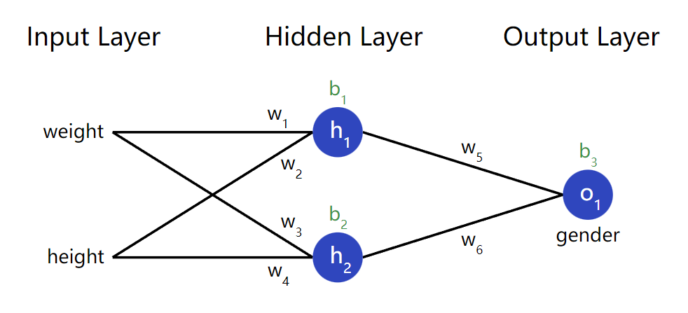
然后,我们可以将损失写成一个多变量函数:
$$
L(w_1, w_2, w_3, w_4, w_5, w_6, b_1, b_2, b_3, b_4)
$$
想象一下,$$w_1$$的值发生改变, 会对损失$$L$$造成什么影响呢?损失$$L$$应该怎么变化呢?在换句话说,这个损失$$L$$,由$$w_1$$贡献了多少呢?这里就会用到偏导数: $$\frac{\partial{L}}{\partial{w_1}}$$。
具体如何计算损失呢?
这里计算会相对复杂一些,但这也是神经网络的核心,花点时间,使用纸笔画一画,帮助理解。
让我们使用链式法则把$$\frac{\partial{L}}{\partial{w_1}}$$变一下形:
$$
\frac{\partial{L}}{\partial{w_1}} = \frac{\partial{L}}{\partial{y_{pred}}} * \frac{\partial{y_{pred}}}{\partial{w_1}}
$$
其中$$\frac{\partial{L}}{\partial{y_{pred}}}$$我们已经可以计算了,因为在前面已经计算过$$L = (1 - y_{pred})^2$$,那么$$\frac{\partial{L}}{\partial{y_{pred}}}$$:
$$
\frac{\partial{L}}{\partial{y_{pred}}} = \frac{\partial{(1 - y_{pred})^2}}{\partial{y_{pred}}} = \boxed{-2(1 - y_{pred})}
$$
然后,我们要考虑如何计算$$\frac{\partial{y_{pred}}}{\partial{w_1}}$$。和前面的方式一样,我们让$$h_1, h_2, o_1$$作为神经元的输出:
$$
y_{pred} = o_1 = f(w_5 h_1 + w_6 h_2 + b_3) \\
这里的激活函数f是sigmoid函数
$$
再然后,由于$$w_1$$只会影响到$$h_1$$,因此我们再继续使用链式法则将$$\frac{\partial{y_{pred}}}{\partial{w_1}}$$变一下形:
$$
\frac{\partial{y_{pred}}}{\partial{w_1}} = \frac{\partial{y_{pred}}}{\partial{h_1}} * \frac{\partial{h_1}}{\partial{w_1}}
$$
$$
\frac{\partial{y_{pred}}}{\partial{h_1}} = \boxed{w_5 * f’(w_1 x_1 + w_2 x_2 + b_1)}
$$
继续,对$$\frac{\partial{h_1}}{\partial{w_1}}$$链式法则:
$$
h_1 = f(w_1 x_1 + w_2 x_2 + b1)
$$
$$
\frac{\partial{h_1}}{\partial{w_1}} = \boxed{x1 * f’(w_1 x_1 + w_2 x_2 + b1)}
$$
上式中,$$x_1$$是体重,$$x_2$$是身高。然后,我们推导$$f’(x)$$,因为已经看到两次了。它本质是有sigmoid激活函数来的:
$$
f(x) = \frac{1}{1 + e^{-x}} \
f’(x) = \frac{e^{-x}}{(1 + e^{-x})^2} = \boxed{f(x) * (1 - f(x)}
$$
后续会使用到$$f’(x)$$的等价公式。
最后,我们成功将$$\frac{\partial{L}}{\partial{w_1}}$$使用链式法则,分解为了几个部分,让我们可以计算:
$$
\boxed{\frac{\partial{L}}{\partial{w_1}} = \frac{\partial{L}}{\partial{y_{pred}}} * \frac{\partial{y_{pred}}}{\partial{h_1}} * \frac{\partial{h_1}}{\partial{w_1}}}
$$
这个神经网络系统中,从最右边的输出层得到的损失函数,向最左边的输入层计算偏导的过程(从右向左进行计算,注意和前馈的概念分开),我们称之为反向传播(backpropagation,简称BP算法)
前馈神经网络的训练方法有很多,使用BP算法进行训练的前馈神经网络,又叫做BP网络(效果好,受欢迎)。
其它常见的前馈神经网络,还有比如感知机网络、径向基函数(Radial Basis Function, RBF)网络,仅做了解。
好了,虽然有很多公式,可能有点绕,但下面直接通过一个例子来看具体是怎么计算这些偏导的吧!
例子:计算偏导
这里继续使用前面Alice的例子作为我们的数据集:
| Name | Weight (minus 135) | Height (minus 66) | Gender |
|---|---|---|---|
| Alice | -2 | -1 | 1 |
然后我们初始化所有的权重$$w$$为1,所有的偏置$$b$$为0。然后我们做一次前向传播,经过神经网络后,得到:
$$
\begin{align}
h_1 &= f(w_1 x_1 + w_2 x_2 + b_1) \
&= f(-2 + -1 + 0) \
&= 0.0474
\end{align}
$$
$$
h_2 = f(w_3 x_1 + w_4 x_2 + b_2) = 0.0474
$$
$$
\begin{align}
o_1 &= f(w_5 h_1 + w6 h_2 + b_3) \
&= f(0.0474 + 0.0474 + 0) \
&= 0.524
\end{align}
$$
因此,计算得到神经网络的预测输出为$$y_{pred} = 0.524$$,这表示没有对性别没有一个明显的偏向,既有可能为男生(0),也有可能为女生(1)。这样正常,因为这个网络还没有经过训练(学习),给出的预测结果并不好。
让我们计算偏导$$\frac{\partial{L}}{\partial{w_1}}$$:
$$
\boxed{\frac{\partial{L}}{\partial{w_1}} = \frac{\partial{L}}{\partial{y_{pred}}} * \frac{\partial{y_{pred}}}{\partial{h_1}} * \frac{\partial{h_1}}{\partial{w_1}}}
$$
$$
\begin{align}
\frac{\partial{L}}{\partial{y_{pred}}} = \frac{\partial{(1 - y_{pred})^2}}{\partial{y_{pred}}} &= \boxed{-2(1 - y_{pred})} \
&= -2 (1 - 0.524) \
&= -0.952
\end{align}
$$
$$
\begin{align}
\frac{\partial{y_{pred}}}{\partial{h_1}} &= \boxed{w_5 * f’(w_1 x_1 + w_2 x_2 + b_1)} \
&= 1 * f’(0.0474 + 0.0474 + 0) \
&= f(0.0948) * (1 - f(0.0948)) \
&= 0.249
\end{align}
$$
$$
\begin{align}
\frac{\partial{h_1}}{\partial{w_1}} &= \boxed{x1 * f’(w_1 x_1 + w_2 x_2 + b1)} \
&= -2 * f’(-2 + -1 + 0) \
&= -2 * f’(-3) * (1 - f(-3)) \
&= -0.0904
\end{align}
$$
$$
\begin{align}
\frac{\partial{L}}{\partial{w_1}} &= -0.952 * 0.249 * -0.904 \
&= \boxed{0.0214}
\end{align}
$$
其中f’(x)的计算在上文中推导过,就是sigmoid激活函数的导数:$$f’(x) = \frac{e^{-x}}{(1 + e^{-x})^2} = \boxed{f(x) * (1 - f(x)}$$
这里也能看出来,如果我们增加权重$$w_1$$,损失函数$$L$$最后会出现一点增长。换句话说,$$w_1$$对最后损失函数$$L$$的贡献度是正的0.0214。
训练:随机梯度下降法
有了上面的基础,我们可以使用很多优化算法可以使用来训练我们的网络。这里我们使用随机梯度下降法(Stochastic Gradient Descent, SGD)来优化改变我们的权重和偏置,最后使我们的损失$$L$$最小。(简单易懂,效果不错)
基本上,对$$w_1$$的更新等式:
$$
w_1 \leftarrow w_1 - \eta \frac{\partial{L}}{\partial{w_1}}
$$
其中,$$\eta$$是一个设定的常数,称之为学习率(Learning Rate, LR),这个设定的常数可以控制我们训练的速度。上式的意思就是说,在原来的$$w_1$$ 基础上,减去$$\eta \frac{\partial{L}}{\partial{w_1}}$$,最后得到一个新的$$w_1$$。
- 如果$$\frac{\partial{L}}{\partial{w_1}}$$是正的,$$w_1$$将变小,进一步会使损失$$L$$减少(在下次训练的时候)。
- 如果$$\frac{\partial{L}}{\partial{w_1}}$$是负的,$$w_1$$将增大,进一步也会使损失$$L$$减少(在下次训练的时候)。
如果我们对网络中的每个权重和偏置都做相同的运算,那损失将慢慢减少,最后使我们的神经网络得到改善。
总结,我们的整个训练过程将会如下所示:
- 从我们的数据集中选择一个样本,一次只对一个样本进行操作。
- 计算损失$$L$$对所有的不同权重或偏置求偏导数。(比如,原始的$$L(w_1, w_2, w_3, w_4, w_5, w_6, b_1, b_2, b_3, b_4)$$,对其每个变量求偏导$$\frac{\partial{L}}{\partial{w_1}}, \frac{\partial{L}}{\partial{w_2}}, \frac{\partial{L}}{\partial{w_3}}……$$)
- 使用上面类似的更新公式,来更新每个权重和偏置。
- 返回到步骤1。
不断重复步骤1-4,就是一个不断训练的过程。
OK,下面将理论推导转化为实际的代码。
编写:一个完整的神经网络
终于,我们可以编写一个完整的神经网络了,同样,继续使用前面的数据集:
| Name | Weight (minus 135) | Height (minus 66) | Gender |
|---|---|---|---|
| Alice | -2 | -1 | 1 |
| Bob | 25 | 6 | 0 |
| Charlie | 17 | 4 | 0 |
| Diana | -15 | -6 | 1 |
继续使用前面的神经网络结构:
1 | import numpy as np |
最后结果可以看到:随着网络的学习,我们的损失逐步减少:

使用训练好的网络,再来进行性别预测:
1 | # Make some predictions |
最后,可以看到我们的神经网络已经能比较正确分辨体重和身高特征较为明显的男生女生。
Reference
PCA,SVD: 矩阵运算,旋转拉伸。
CNN: 卷积、信号处理、傅里叶变换。